Deep learning is cool and for applications like image processing and speech understanding has truly raised the bar but if you want to win a Kaggle competition you might want to check out Gradient Boosted Decision Trees (GBDTs) like Xgboost [code] from Tianqi Chen or new contender from Microsoft LightGBM [code].

What are the things that make GBDT attactive?

1. They can learn the important crosses between input variables by incorporating them into trees.
2. They require minimal data processing before inputting data. No normalization is required since they use ranks of data rather than values themselves.
3. Implementations like XGBoost and LightGBM can be trained in a distributed fashion on large datasets quickly.
4. Lots of parameters to regularize and tune performance.

Some downsides to GBDTs are:

1. Only can classify numerical data, isn’t always clear how to best encode categorical data for learning with a GBDT.
2. Unlike neural nets they don’t generate any internal represenation of features (embeddings) for kNN or other applications.
3. Can’t train online like logistic regression, there is no SGD for GBDTs.

Some details on the magical model

XGBoost like many classification approaches models the objective function (cost) to minimize as a combination of the loss \(L(\theta)\) for a set of parameters and the regularization penalty $\Omega(\theta)$ for having a complex parameter set.

\[ \text{obj}(\theta) = L(\theta) + \Omega(\theta) \]

The model is of the form:

\[ \hat{y}\_i = \sum\_{k=1}^K f\_k(x\_i), f\_k \in \mathcal{F} \]

where $(K)$ is the number of trees, $f$ is a function in the functional space $\mathcal{F}$, and $\mathcal{F}$ is the set of all possible Classification And Regression Trees (CARTs_. Therefore our objective to optimize can be written as:

$$ \text{obj}(\theta) = \sum\_i^n l(y\_i, \hat{y}\_i) + \sum\_{k=1}^K \Omega(f\_k) $$

It is a little mind bending coming from linear models to have a parameterization of functions $f$ over a function space $\mathcal{F}$. It isn’t possilble to evaluate all possible trees so GBDTs rely on heuristics to build up promising solutions over the space. Trees are built additively over time with more trees

$$ \begin{split}\hat{y}_i^{(0)} &= 0\\ \hat{y}_i^{(1)} &= f_1(x_i) = \hat{y}_i^{(0)} + f_1(x_i)\\ \hat{y}_i^{(2)} &= f_1(x_i) + f_2(x_i)= \hat{y}_i^{(1)} + f_2(x_i)\\ \dots\\ \hat{y}_i^{(t)} &= \sum_{k=1}^t f_k(x_i)= \hat{y}_i^{(t-1)} + f_t(x_i) \end{split} $$

So which trees get added? Here we are going to greedily add the one that optimizes our objective function. Specifically:

$$ \begin{split}\text{obj}^{(t)} = \sum_{i=1}^n l(y_i, \hat{y}_i^{(t)}) + \sum_{i=1}^t\Omega(f_i) \\ = \sum_{i=1}^n l(y_i, \hat{y}_i^{(t-1)} + f_t(x_i)) + \Omega(f_t) + constant \end{split} $$

The squared loss MSE differentiates nicely. Some of the other loss functions like logistic loss aren’t as nice in this formulation, so XGBoost approximates with the first couple terms of the Taylor series.

$$ \text{obj}^{(t)} = \sum_{i=1}^n [l(y_i, \hat{y}_i^{(t-1)}) + g_i f_t(x_i) + \frac{1}{2} h_i f_t^2(x_i)] + \Omega(f_t) + constant $$

where

$$ \begin{split} g_i= \partial_{\hat{y}_i^{(t-1)}} l(y_i, \hat{y}_i^{(t-1)})\\ h_i = \partial_{\hat{y}_i^{(t-1)}}^2 l(y_i, \hat{y}_i^{(t-1)}) \end{split} $$

To model the complexity they need a good definition of the tree.

$$ f_t(x) = w_{q(x)}, w \in R^T, q:R^d\rightarrow \{1,2,\cdots,T\} $$$$ \Omega(f) = \gamma T + \frac{1}{2}\lambda \sum_{j=1}^T w_j^2 $$

Then XGBoost uses some fancy math to define what would be a great cut

$$ \begin{split} \text{obj}^{(t)} \approx \sum_{i=1}^n [g_i w_{q(x_i)} + \frac{1}{2} h_i w_{q(x_i)}^2] + \gamma T + \frac{1}{2}\lambda \sum_{j=1}^T w_j^2\\ = \sum^T_{j=1} [(\sum_{i\in I_j} g_i) w_j + \frac{1}{2} (\sum_{i\in I_j} h_i + \lambda) w_j^2 ] + \gamma T \end{split} $$

where $I_j = \{i|q(x_i)=j\} $ is the set of indices of data points assigned to the $j$-th leaf. Note that in the second line they have changed the index of the summation because all the data points on the same leaf get the same score. For notation they could further compress the expression by defining $G_j = \sum_{i\in I_j} g_i$f and $H_j = \sum_{i\in I_j} h_i$ So then

$$ \text{obj}^{(t)} = \sum^T_{j=1} [G_jw_j + \frac{1}{2} (H_j+\lambda) w_j^2] +\gamma T $$

Pulling in some tricks related to the best solution for a quadratic equation as $w_j$ are independent with respect to each other, the form $G_jw_j+\frac{1}{2}(H_j+\lambda)w_j^2$ is quadratic and the best $w_j$ for a given structure $q(x)$ and the best objective reduction possible is:

$$ \begin{split} w_j^\ast = -\frac{G_j}{H_j+\lambda}\\ \text{obj}^\ast = -\frac{1}{2} \sum_{j=1}^T \frac{G_j^2}{H_j+\lambda} + \gamma T \end{split} $$

So the gain of making a cut is the score of the new leaf on the left, the score of leaf on the right minus the score on the original leaf and a regularization term at the end.

$$ Gain = \frac{1}{2} \left[\frac{G_L^2}{H_L+\lambda}+\frac{G_R^2}{H_R+\lambda}-\frac{(G_L+G_R)^2}{H_L+H_R+\lambda}\right] - \gamma $$

Tuning

XGBoost has a whole page on the knobs that can be tuned but many of them are familiar from the equations above:

• eta $\eta$ step size shrinkage used in update to prevent over fitting.
• gamma $\gamma$ minimum loss reduction required to make another partition on a leaf node of the tree
• max_depth maximum size of trees
• subsample only collect some of the dat instances to grow trees.
• lambda L2 regularization on weights
• alpha L1 regularization on weights.

And a number of other ones to checkout for tuning as everyone loves to play with hyperperameters to squeeze out the last bits.

What is new in LightGBM?

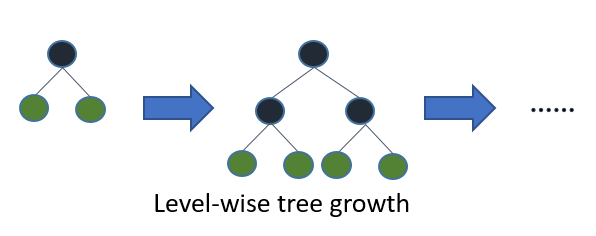
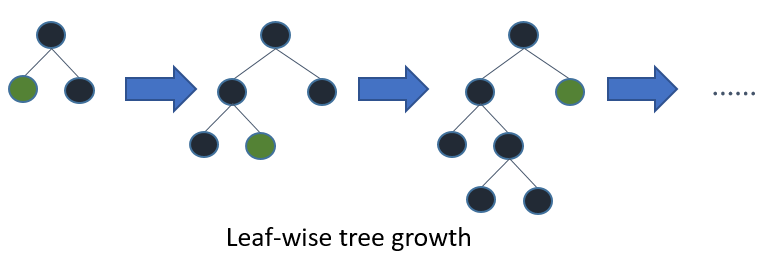
Ke et al. have sped up their implementation significantly by being more sophisiticated about how they sample and how the pick features to do splits. on. Specifically they show that their Gradient based One-Side Sampling (GOSS) and Exlusive Feature Bundling (EFB) can greedily discard many sub standard trees and still be a good approximation to the NP-hard version of bundling exclusive features. In short they go even faster. LightGBM can also model slightly more complex trees as they grow them per leaf rather than per level.